About Hard and Soft Iron Distortions .
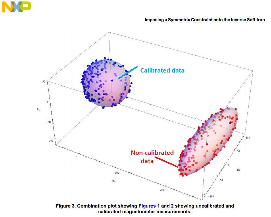
Magnetic measurements will be subjected to distortion. These distortions are considered to fall in one of two categories; hard or soft iron. Hard iron distortions are created by objects that produce a magnetic field. A speaker or piece of magnetized iron for example will cause a hard iron distortion. If the piece of magnetic material is physically attached to the same reference frame as the sensor, then this type of hard iron distortion will cause a permanent bias in the sensor output. Soft iron distortions are considered deflections or alterations in the existing magnetic field. These distortions will stretch or distort the magnetic field depending upon which direction the field acts relative to the sensor. This type of distortion is commonly caused by metals such as nickel and iron. In most cases hard iron distortions will have a much larger contribution to the total uncorrected error than soft iron.
Learn more about them :
- https://www.sensorsmag.com/components/compensating-for-tilt-hard-iron-and-soft-iron-effects
- https://www.nxp.com/docs/en/application-note/AN4246.pdf
Using Artificial Intelligence for magnetometer calibration on ESPrtk .
ESPrtk's calibration quality is very high.
ESPrtk version 3.9.8 uses artificial intelligence (AI) to solve noise removal and automatically find the calibration matrix very accurately.
It has been tested many times with different data inputs (a lot of noise, missing spherical data) and both solved them perfectly.
Using AI solves problems that old algorithms cannot solve such as determining eccentricity and distortion with noisy input data samples (or simply being unable to determine where 'standard shape' of the input data).
The result was astonishing, with 99.99% eliminated noise. The algorithm works very well, even when only 1/4 surface points data exist in input data. Distortion and eccentricity due to hard-iron and soft-iron are completely removed.
Testing results.
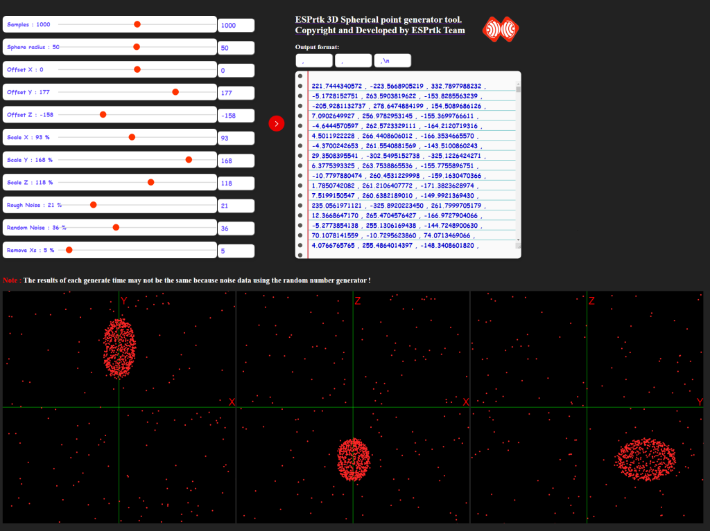
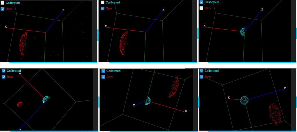
During the development of AI calibration algorithm for ESPrtk. We wrote a program to create different data samples with real-world effects such as deformation of hard iron and soft iron, noise, roughness, duplicate pattern, etc.
You can also download it here: Link Download
For more using magnetometer calibration tool on ESPrtk, go to this page .
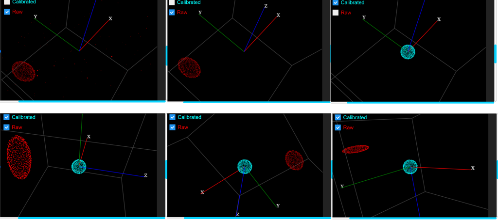
Below are some capture images of the calibration results.
Exam 1.
| Configure | Value | Configure | Value |
|---|---|---|---|
| Samples | 1000 | Offset X | -244 |
| Sphere radius | 50 | Offset Y | 200 |
| Rough Noise | 9 % | Offset Z | -155 |
| Random Noise | 20 % | Scale X | 100 % |
| Remove_Y_axis | 0% | Scale Y | 152 % |
| Download | Link | Scale Z | 40 % |
Exam 4.
| Configure | Value | Configure | Value |
|---|---|---|---|
| Samples | 1000 | Offset X | -220 |
| Sphere radius | 50 | Offset Y | 150 |
| Rough Noise | 11 % | Offset Z | -223 |
| Random Noise | 80 % | Scale X | 151 % |
| Remove_Y_axis | 0 % | Scale Y | 53 % |
| Download | Link | Scale Z | 200 % |
Exam 6.
| Configure | Value | Configure | Value |
|---|---|---|---|
| Samples | 1000 (removed 1/2 sphere surface X-axis ) | Offset X | 160 |
| Sphere radius | 50 | Offset Y | 152 |
| Rough Noise | 8 % | Offset Z | 206 |
| Random Noise | 28 % | Scale X | 65 % |
| Remove_Y_axis | 50 % | Scale Y | 135 % |
| Download | Link | Scale Z | 61 % |
Exam 7.
| Configure | Value | Configure | Value |
|---|---|---|---|
| Samples | 1000 (removed 1/2 sphere surface Y -axis ) | Offset X | 132 |
| Sphere radius | 49 | Offset Y | -158 |
| Rough Noise | 2 % | Offset Z | 146 |
| Random Noise | 20 % | Scale X | 100 % |
| Remove_Y_axis | 50 % | Scale Y | 200 % |
| Download | Link | Scale Z | 100 % |
Exam 8.
| Configure | Value | Configure | Value |
|---|---|---|---|
| Samples | 1167 (removed 3/4 sphere surface Y -axis ) | Offset X | -112 |
| Sphere radius | 50 | Offset Y | 152 |
| Rough Noise | 0 % | Offset Z | -137 |
| Random Noise | 5 % | Scale X | 100 % |
| Remove_Y_axis | 75 % | Scale Y | 200 % |
| Download | Link | Scale Z | 100 % |
About Hard and Soft Iron Distortions .
Magnetic measurements will be subjected to distortion. These distortions are considered to fall in one of two categories; hard or soft iron. Hard iron distortions are created by objects that produce a magnetic field. A speaker or piece of magnetized iron for example will cause a hard iron distortion. If the piece of magnetic material is physically attached to the same reference frame as the sensor, then this type of hard iron distortion will cause a permanent bias in the sensor output. Soft iron distortions are considered deflections or alterations in the existing magnetic field. These distortions will stretch or distort the magnetic field depending upon which direction the field acts relative to the sensor. This type of distortion is commonly caused by metals such as nickel and iron. In most cases hard iron distortions will have a much larger contribution to the total uncorrected error than soft iron.
Learn more about them :
- https://www.sensorsmag.com/components/compensating-for-tilt-hard-iron-and-soft-iron-effects
- https://www.nxp.com/docs/en/application-note/AN4246.pdf
Using transformation matrix on ESPrtk.
Steps to calibrate magnetometer on ESPrtk .
Step1 : Get the raw data (text file).
Input of software is a text file containing raw data on 3 axes of XYZ magnetometer.
Step2: Find transform matrix using Magneto1.2.
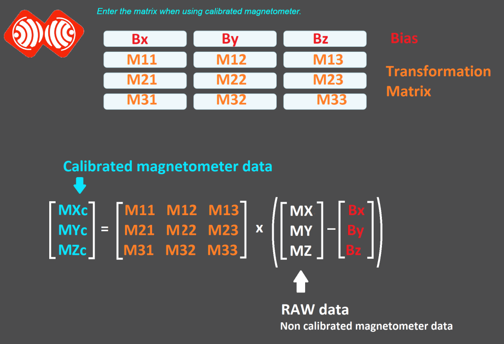
Find hard iron compensation (Bias) and soft iron compensation (matrix M [3,3] ) from the raw data file.
Download Magneto1.2 here :
- Magneto12_Calibration_Helper ESPrtk — (ESP Cloud)
- Sample rate :10 Hz
- Max sample : 1000. (or more)
- File format exxport : .txt
- Data output format : Using default configure . (X Y Z + Enter)
Step3 : Applying transformation matrix and Check calibrated data.
Wiring MPU9250 to use with ESPrtk
See the circuit diagram here : IMU-MPU9250 Export IMU data in Real time.
Step1 : Get the raw data (text file).
Learn how to use ‘Calibration Helper’ here: IMU MPU9250 Calibration Helper .
The file format requires values separated by 1 White space character (‘ ‘) and ends with 1 new line character (‘\n’) for each sample.
Configure :
Step2: Find transform matrix using Magneto1.2.
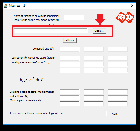
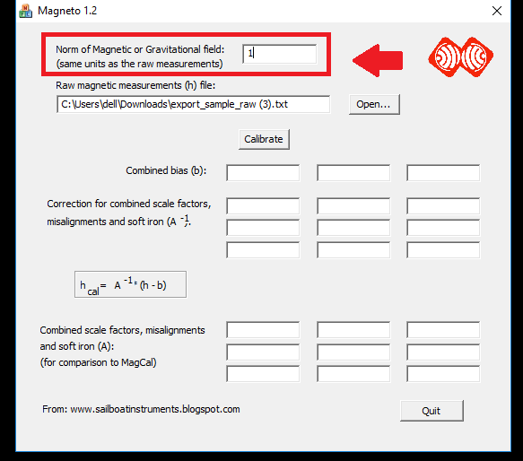
Click ‘Open’ and find file named ‘export_sample_raw.txt’.
Enter ‘Norm’ value before calibrate. Usually start with ‘1’.
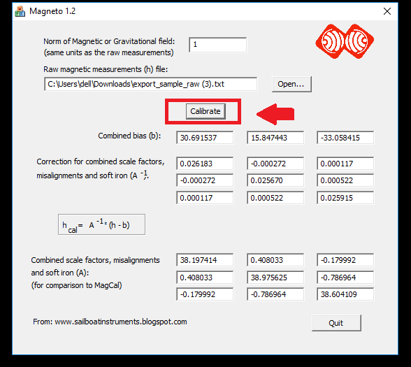
Press ‘Calibrate’ button to start calculate.
The ‘Norm’ value will use for scale the matrix output.
And the values of main diagonal must equal or approximately equal to ‘1’.
Increasing or decreasing Norm’s value will help find the best main diagonal for transformation matrix.
In this case . Norm is ‘1’ and the main diagonal is [0.026183 , 0.025670,0.025915] .
Increasing Norm to ’10’ and the main diagonal is [0.26183 , 0.25670,0.25915] , they are closer to 1 but the difference is still too large.
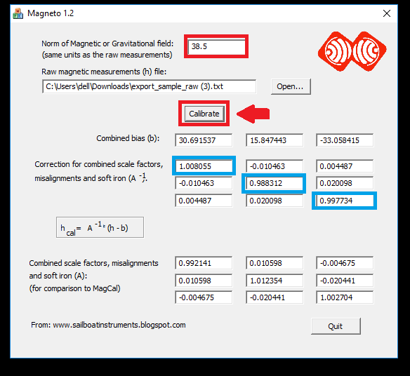
After a few times of adjusting the value, the best Norm value in this case is 38.5.
And the main diagonal is [1.008 , 0.988 , 0.997 ] , approximately equal to ‘1’.
Note : Dont type Enter on Norm field , that will make the software crash.!
See a video below :
Step3 : Applying transformation matrix and Check calibrated data.
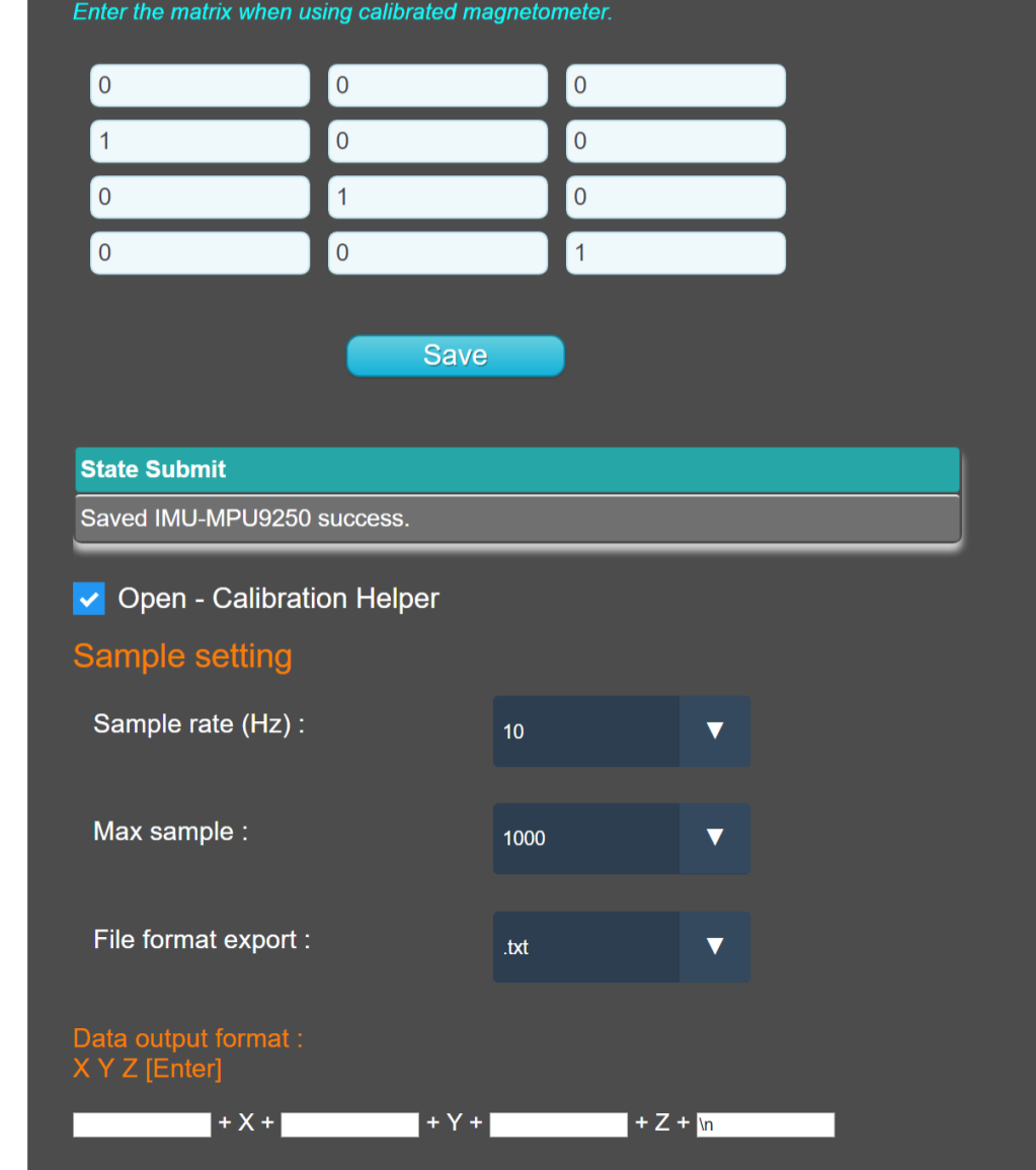
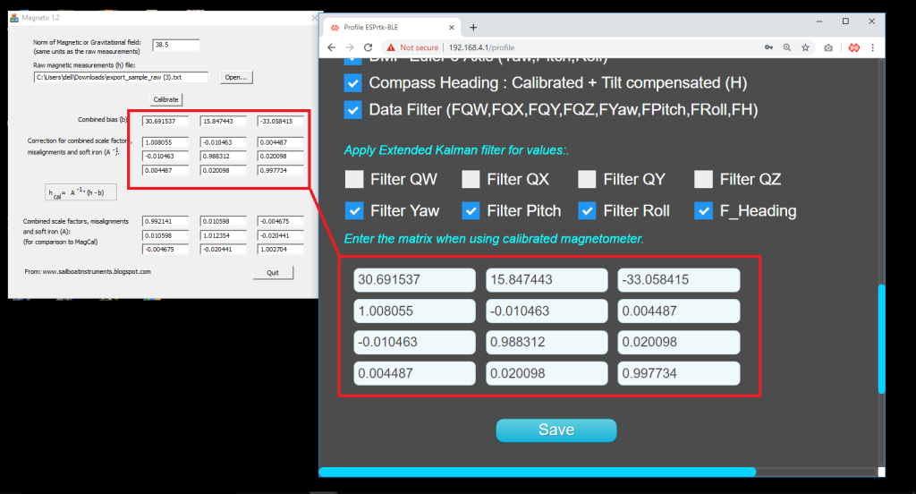
Now , go back to IMU-MPU9250 tab on ESPrtk and enter to the matrix and press ‘Save’ .
Open ‘Calibration Helper’ and rotate again sensor to evaluate the effect of applying the matrix to calibration.
See videos below :
